


Data is the brain of online marketing. Your business can jump into a nightmare, and be in trouble when running an eCommerce business with thousands of SKUs. However, the profit margin calculation is being messed up. It is critical to make things in order and in place well. It’s because this calculation is associated with the selling price and different variable costs that can cause a business loss in the end.
In this article, I’ll introduce 9 Google Sheet formulas + 1 automation add-on for your eCommerce marketing operation. By the end of the article, you could learn about my practical experience on how to apply these Google sheet formulas, functions, and add-ons to set your hands free and calculate accurately.
- IF ( )
- IFERROR ( )
- INDEX ( )
- MATCH ( )
- MAX ( )
- MIN ( )
- SUMPRODUCT ( )
- ROUNDUP ( )
- SUMIFS ( )
- ADD-ONS SUPERMETRICS
1. IF()
The IF function runs a logical test and returns one value for a TRUE result, and another for a FALSE result. The syntax is here:
=IF (logical_test, [value_if_true], [value_if_false]).
Take Amazon FBA fee calculation as an example
The fulfillment fee varies depending on the product size and shipping weight of the item being shipped. There are 4 standards:
Small standard size, Large (<1lb)Standard size, Large (1-2lbs) Standard size, Large (>2lb) standard size.
Let us see how to use the IF function to calculate all of the SKUs automatically.
Step 1: Identify which standard size range the SKU falls into
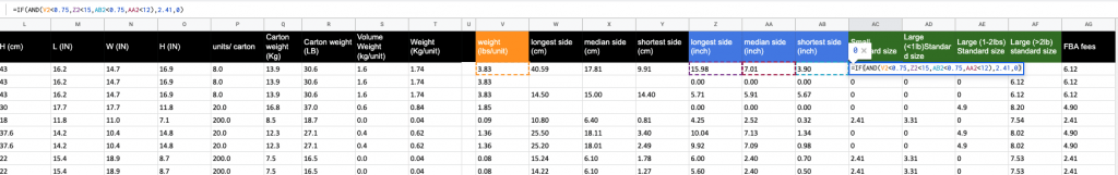

Each standard size has its range of shortest side (inch), longest side (inch), median side (inch), and weight (lbs/unit). For instance, a small standard size SKU is less than 0.75 lbs/unit. The longest side is less than 15 inches. The median side is less than 0.75 inches, and the shortest side is less than 12 inches. An SKU is under the small standard size if 4 conditions meet the requirement, and the FBA fee is US$2.41
So we could automate the resting of the SKU FBA fee calculation by using these Google Sheet formulas. (Sample)
=IF(AND(V2<0.75,Z2<15,AB2<0.75,AA2<12),2.41,0)
Note: IF with AND states the result needs to meet all arguments in the formula)
Step 2: Choose the smallest size
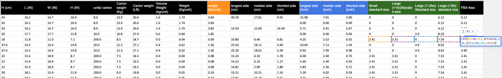

As you can see from the results in step 1, some smaller SKUs can have 2, or even 4 FBA fees. For instance, small standard size, and large standard size. The reason is when an SKU size is pretty small, it locates in the lowest standard size. Also, it can be within all resting of higher requirements as well. However, in fact, we won’t ship a smaller piece by using a larger size rate.
The IF function can be “nested“. A “nested IF” refers to a formula where at least one IF function is nested inside another in order to test for more conditions and return more possible results. Each IF statement needs to be carefully “nested” inside another so that the logic is correct.
So we could automate choosing the smallest size rate, or cheapest by using Google Sheet formulas. (Sample)
=IF(AC6>0,AC6,IF(AD6>0,AD6,IF(AE6>0,AE6,AF6)))
2. IFERROR()
IFERROR returns a custom result when a formula generates an error. It generates a correct result when no error is detected in Google sheet functions. IFERROR is an elegant way to trap and manage errors, and the syntax is here:
IFERROR( formula, alternate_value).
Take Amazon FBA fee calculation as an instance again.
In the IF formulate which is used to Identify which standard size range the SKU falls into, either V2, AB2, and AA2 return a string or #error, any SKU FBA fee calculation results in #error as well.
Google Sheet Formulas (Sample)
=IF(AND(V2<0.75,Z2<15,AB2<0.75,AA2<12),2.41,0)
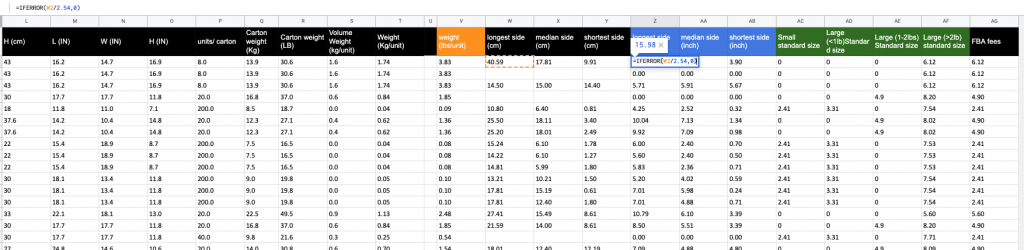

As you can see from the table, we know this SKU’s longest side cm is 40.59, and this number needs converting into an inch unit. For avoiding any error appearing, we can use the IFERROR formula and return 0 if the error comes up.
=IFERROR(W2/2.54,0)
3 & 4. INDEX() and MATCH()
INDEX and MATCH is the most popular tool in Google Sheet functions for performing more advanced lookups. This is because INDEX and MATCH are incredibly flexible – you can do horizontal and vertical lookups, 2-way lookups, left lookups, case-sensitive lookups, and even lookups based on multiple criteria. This is the syntax:
INDEX(array, row_num, [column_num])
MATCH(lookup_value, lookup_array, [match_type])
Take profit and loss modeling as an example
Amazon FBA fee is a type of variable cost, and the FBA cost needs using on the SKU profit calculator, so you can calculate and see what’s the profit of the SKU minus the FBA fees.
The question is how to find the FBA fee value to a specific SKU in the profit margin calculator spreadsheet? The answer is you can use the combination of the index and match function.
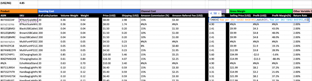

Google Sheet Formulas
=INDEX('Raw per SKU'!$AG$2:$AG$1052,match(B5,'Raw per SKU'!$A$2:$A$1052,0))
First of all, you use INDEX to navigate the area which has the value you’re seeking for the SKU profit calculation in the P&L spreadsheet. As you can see, it is ‘Raw per SKU’!$AG$2:$AG$1052
Secondly, you use the match function to calibrate the SKU you’re looking up, which is BTNutrScaleBkUSA, and is added to the 1st argument. Then, the SKU area in the raw per SKU tab is needed as well which is added to the array argument. Lastly, 0 is added if the exact match type is applicable.
Last but not least, please remember to set an absolute value on the INDEX array, and match the array by ctrl + F4.
5 & 6. MAX() & MIN()
To find the lowest value in a range of cells, use the MIN function. On the other hand, to find the highest value in a range of cells, use the MAX function. The syntax is:
=MIN(number1, [number2],….)
=MAX(number1, [number2],….)
Or the ‘number’ can be keyed directly into the formula, or you can enter a cell range (e.g. B15:F15).
Take sourced product shipment as an instance
Most sellers source the product from Asian countries, such as China, and basically, the manufacturers ship the sourced products to your warehouse of the targeted market. FBA fees won’t include the shipment part from China to your targeted market. So you need to plug this shipping fee in your profit calculator.
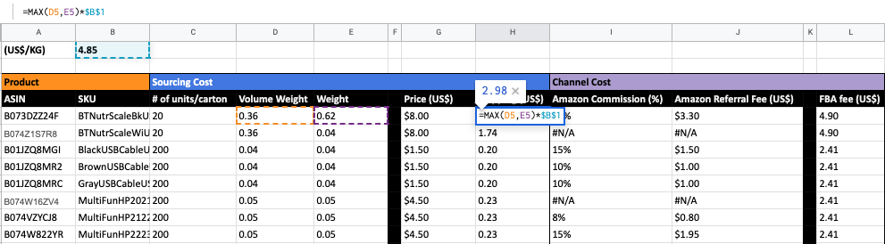

However, the argument is that there’re two types of weight – actual weight and volume weight, from a logistic perspective. Actual weight is determined by the heaviness, or mass, of the particular item, and is measured with the use of a scale. The volume weight is the amount of space that an item you are measuring takes up. So you can use Max or Min function to choose the value in the shipping cost.
=MAX(D5,E5)*$B$1
Normally, for leaving more buffer, you can select MAX, which you prefer the bigger weight between them.
7. SUMPRODUCT()
The SUMPRODUCT function multiplies ranges or arrays together and returns the sum of products. This sounds boring, but SUMPRODUCT is an incredibly versatile function that can be used to count and sum like COUNTIFS or SUMIFS, but with more flexibility. Other functions can easily be used inside SUMPRODUCT to extend functionality even further. The syntax is
=SUMPRODUCT (array1, [array2], ...).
Take eCommerce new product bundling price and cost calculation as an instance
Product bundling is offering several products or services for sale as one combined product or service package. In Google Sheets, you can create a core product, for an instance, an iPhone in a row. This row includes the product selling price and cost. Meanwhile, you can add different product SKUs that are considered to add to bundle with iPhone, for example, the case, the headphone, etc in columns. As you can see from the table below, each column includes the SKU selling price and cost as well.
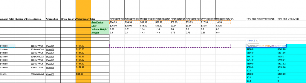

From L68:AI68, you can add the number value of the SKUs that will be bundled with an iPhone. From $L$9:$AI$9, it is the individual SKU retail selling pricing. So if you want to calculate the new bundling retail price value, you can add the array $L$9:$AI$9, and L68:AI68 in the SUMPRODUCT function, plus the iPhone retail price E68.
=sumproduct($L$9:$AI$9,L68:AI68)+$E68
With the same methodology, you can calculate the new bundling product cost, etc as well. However, you need to set up an absolute value reference on $L$9:$AI$9, when you match other iPhone models with the set of accessories.
8. ROUNDUP()
ROUNDUP returns a number rounded up to a given number of decimal places in Google Sheet Functions. Unlike standard rounding, where numbers less than 5 are rounded down, ROUNDUP rounds all numbers up. The syntax is
=ROUNDUP (number, num_digits)
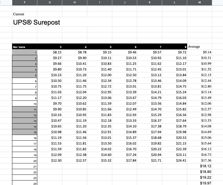
Take eCommerce Self-fulfillment as an instance.
Except for FBA fulfillment, you can use a delivery service provider like UPS, FedEx, etc. As you can see from the below table that is an iPhone device courier rate based on the lbs.

I assume the product bundling is iPhone plus headset, so first of all, you need to calculate both devices’ volume weight, and actual weight, and use the MAX function to choose the bigger weight.
sum(max(AR85:AS85),max(AP85:AQ85))
However, the resulting number has a decimal position, and the UPS rate is different from lbs, which shows in an integer number. So ROUNDUP can help you convert the decimal position automatically into an integer number
roundup(sum(max(AR85:AS85),max(AP85:AQ85)),0).
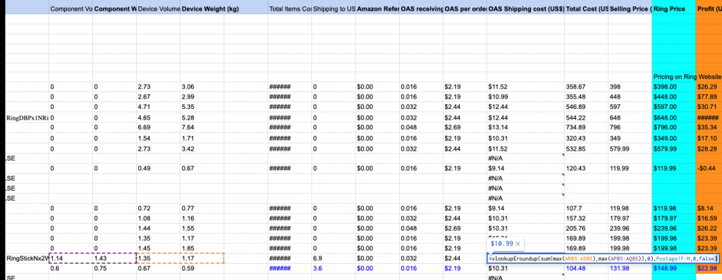

Secondly, the value from this result of the roundup function is a number, that can work with Vlookup’s first argument (The lookup value). By using the formula below, you can return the avg. the shipping fees of both devices by using UPS.
Google Sheet Formulas (Sample)
=vlookup(roundup(sum(max(AR85:AS85),max(AP85:AQ85)),0),Postage!F:M,8,false)
9. SUMIFS()
SUMIF function returns the sum of cells that meet a single condition in Google Sheet functions. Criteria can be applied to dates, numbers, and text. The SUMIF function supports logical operators (>,<,<>,=) and wildcards (*,?) for partial matching. Thy syntax is
=SUMIFS( sum_range, criteria_range1, criteria1, [criteria_range2, criteria2, ... criteria_range_n, criteria_n] )
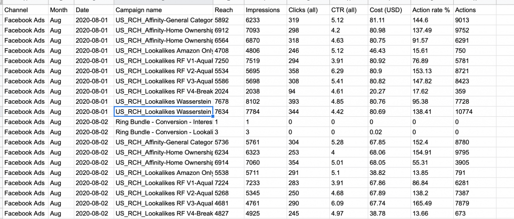
Take lump-sum data from digital marketing platform raw data as an example
eCommerce marketing strategy, like running an omnichannel strategy (Google, Facebook, Instagram, etc), is critical for owners, and marketers to analyze the transaction performance in a simple spreadsheet, that can facilitate connecting with other data sets, rather than analyzing the data from each digital platform separately.
SUMIFS functions help you to summarize the data of whatever information you need in one place from different channels, such as by month by metrics by channel, etc.
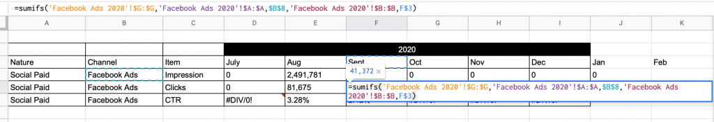
From the table below, it can show Facebook ads performance metrics, such as impressions, clicks, etc, SUMIFS returns these values from an automatic daily monitoring spreadsheet. The pros are you can monitor different SKUs daily, but also the lump-sum performances can update in an automatic way by using SUMIFS Google sheet formulas.
=sumifs('Facebook Ads 2020'!$G:$G,'Facebook Ads 2020'!$A:$A,$B$8,'Facebook Ads 2020'!$B:$B,F$3)


The profit margin calculator can also connect with the digital marketing performance tracker, which is a full picture profit-driven tracker for each SKU
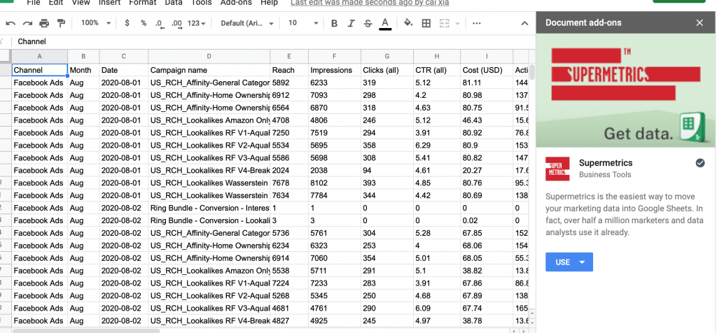
10. Adds-on – Supermetric
Supermetric is easy to use and a powerful data collection tool. You can get any metrics & dimensions from your favorite marketing platforms (DV 360, Facebook, Google, Mailchimp, etc). Also, You can set your reports to refresh automatically. Choose from monthly, weekly, daily, or even hourly refreshes, and then just sit back, relax, and let Supermetrics take care of the heavy lifting. It can work with Google Sheets and data studio as well.

Supermetric has a free trial of 14 days with a fully-featured trial. To access this free trial, simply start using the product in Google Sheets add-ons. Once the trial expires, for some products it will go into a ‘free’ mode where you can continue to use it with some limitations.
Free Plan
Google Sheets: No scheduled refresh, 100 max rows per query, 100 queries per day, Google Analytics only available connector to use
Data Studio: Single assigned user, one ad account per ad network, max date range of last 10 days, only these connectors available to use – Facebook Ads, Twitter Ads, Microsoft Advertising, LinkedIn Ads, MailChimp, Google Analytics, Google Ads, Google Search Console, and Verizon Media Native Ads
BigQuery: No free mode
Excel: No free mode
Uploader: No free mode
Legacy products: No free model
If you are interested in importxml that is used for importing real-time data in Google sheets, please check out this article
Google Sheets ImportXML – Automatically Scrape Web and Collect Product Price Info
I hope you enjoy reading 9 Google Sheet Functions Plus 1 Add-on for the eCommerce Marketing and find it helpful. If you did, please support us by doing one of the things listed below, because it always helps out to our channel.
- Support my channel through PayPal (paypal.me/Easy2digital)
- Subscribe to my channel and turn on the notification bell Easy2Digital Youtube channel.
- Follow and like my page Easy2Digital Facebook page
- Share the article to your social network with the hashtag #easy2digital
- Buy products with Easy2Digital 10% OFF Discount code (Easy2DigitalNewBuyers2020)
- You sign up for our weekly newsletter to receive Easy2Digital latest articles, videos, and discount code on Buyfromlo products and digital software
- Subscribe to our monthly membership through Patreon to enjoy exclusive benefits (www.patreon.com/louisludigital)